Barrier Inside an Infinite Square Well First Excited State Continued

Week 3, lecture 8

Learning objectives

After following this lecture, you will be able to:

• Identify the conditions that lead to bound and scattering states for a given potential.
• Apply the relevant boundary conditions to specify the allowed wavefunctions and energies.
• Recognise symmetries and be able to take advantage of them in order to choose the appropriate method for solving problem.
• Represent graphically the wavefunctions in potentials that combine scattering and bound states.

Finite square well and barrier¶

In the previous lecture, we have discussed an explicit example of a quantum system (the Dirac delta function potential) exhibiting both bound and scattering states.

In this lecture, we are going now to extend this discussion of scattering and bound states to more realistic (and important) configurations in quantum theory, namely systems characterised by either a finite square well or a finite square barrier potentials .

We will first discuss in detail the case of the finite square well potential, and then show how the finite square barrier problem can be extrapolated from the previous case.

Finite square well¶

The finite square well system is defined by the following potentital:

where is a positive real constant that represents how deep is the potential well, and indicates the width of the well. Likewise, the finite square barrier system is defined by

where now represents the height of the potential barrier. As mentioned above, in the following we will focus on the case of the square potential well and then later we will come back to the square barrier case.

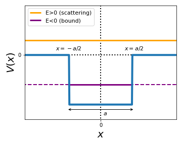
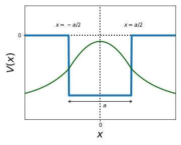
Below we display schematically the potential in the case of the finite square well. Already at the qualitative levelm we can see that this quantum system will admit two types of solutions:

• For we will have scattering states, with a continuum of energies that are not bounded from above. We have that everywhere in space (classically allowed region) and hence for these scattering states we expect an oscillatory behaviour of the wave function.

• For we will have bound states, characterised by a discrete (quantized) energy spectrum and by normalized wavefunctions.

Inside the potential barrier, we have that (solid purple line) and hence we expect an oscillatory behaviour for the wave function. For instead, we are in the classically forbidden regime (dashed purple line) where the wave function is expected to decay exponentially fast and vanish for .

As in the discussion of the delta potential, we start with the bound states and then move to the corresponding scattering states.

Bound states in the finite square well¶

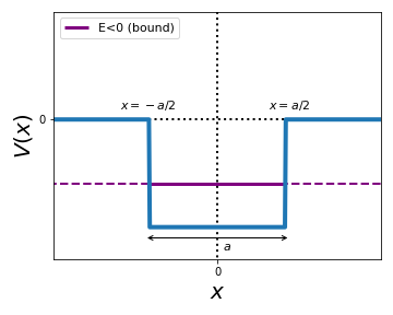
Let's start by discussing bound states in the potential well. For the schematic of the potential displayed below, we can observe that these bound states will have energies in the range . Therefore in the following we consider only solutions whose energies correspond to the situation below, where the solid (dashed) purple line indicates the classically allowed (forbidden) region of .

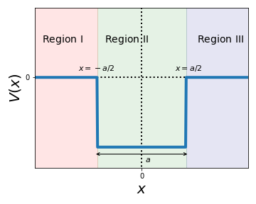
The first step in order to solve the Schroedinger equation in this system is to divide the problem into different regions, with each region having associated a different value of the potential.

It should be clear from the schematic that we need to define three regions: first a region such that where , then the potential well region characterised by , and finally the right part of the potential well where again . These three regions are thus defined by the conditions

and are indicated in the schematic below.

Let us now solve the Schroedinger equation separately in each of the three regions, and relate these solutions by means of the boundary conditions that the wave function of the system must satisfy.

Recall

First, the wave function must be continuous everywhere, so in our case we will impose its continuity at and . Second, we also know that for finite potentials (as in this case) also the first derivative of the wave function must be continuous, and hence we will impose that is continuous at both and .

• :

Here the Schroedinger equation reduces to that of the free particle given that . Therefore the equation that we need to solve in this region is given by

where we have written in the right hand side (RHS) to make explicit the requirement that the energy must be negative there (recall that we are dealing with bound states now).

The most general solution of Eq. [1] will be given by

where as usual and are integration constants that will be fixed by the continuity boundary conditions on the wave function. Note that here we have real (rather than imaginary) exponentials in , as expected given that Region I corresponds to a classically forbidden region.

Furthermore, we know that bound states must have integrable wave functions. To make sure that is finite at , we must impose that . Therefore, we end up finding that the wavefunction in Region I is given by

• :

The Schroedinger equation to be solved in Region III is exactly the same as in Region I, Eq. [1], since in both cases the potential vanishes V(x)=0. Therefore we will have that

and to ensure that the wavefuntion vanishes when (which is required to make the wave function of this bound state normalisable) then we need to impose that and hence we find that in Region III the wave function is given by

with the exponential suppresion characteristic of the quantum wave functions in classically forbidden regions.

• :

Finally, we need to tackle Region II, corresponding to the inside of the potential well, and where the energy satisfies . The Schroedinger equation to be solved in this region is the following:

and moving to the RHS of the equation

Since is positive and (see the schematics above) it follows that , and thus you can verify that the most general solution to Eq. [4] will be given by

which displays an oscillatory behaviour, rather than the real exponentials that characterised the wave functions in Regions I and III.

Recall

Using the expression of the cosinus and the sinus in terms of complex exponentials, and you can show that a linear combination of and can always be expressed as a linear combination of and .

We know that a linear combination of imaginary exponentials can be rewritten as a linear combinations of sinus and cosinus with the same argument; we use this property to express the solution to Eq. [4]: as

.

This transformation, as we will show below, greatly facilitates the physical intepretation of the wave function in this region.

Note also that Eq. [5] is the sum of a symmetric function () and of an antisymmetric function (). This observation will become handy in the following.

We can now put together the wave functions that we have derived in the three regions of this problem:

We see that the solutions obtained depend on four unknown integration constants and . Fortunately, imposing the boundary conditions mentioned above we may be able to fix these some of these constants, since we have two relations coming from imposing the continutity of the wavefunction at and two more from imposing the same condition for the first derivative.

• Continuity of the wavefunction:

From Eq. [6] we derive the following relation between , and :

where note that we have used the symmetry (antisymmetry) property of the cosinus (sinus).

Before moving forward, we note that the potential function of the finite well problem is symmetric, , in other words, it is an even function of the position . This property has an important consequence, which is fully general and applies also beyond this specific system.

Info

A symmetric potential (such that ) imposes certain conditions on the symmetry properties of the wavefunction. If we consider the Schroedinger equation and now we transform from to and use that the potential is symmetric we get that we can conclude that the solutions of this equation must have associated well-defined symmetry properties upon a transformation: they must be either even functions in the position , , or instead odd functions of the position, . Only function with those properties can be solutions of the Schroedinger equation with a symmetric potential.

In our case, since the square well potential is symmetric in Region II, we know that the wave functions in this region, Eq. [5], must be either even or odd functions of : .

Now, this is why it was a good idea to express in terms of sinus and cosinus: for the even solutions, , we will have that (since the sinus is an odd function) while conversely for the odd solutions, , we will have since the cosinus is even.

In the case of the even solutions, imposing reduces Eq. [8] to

and likewise in this case Eq. [7] is simplified to

We will come back later to the case of the odd solutions, for the time being we continue our derivation of the equations imposed by the boundary conditions for the case of even wavefunctions.

• Continuity of the first derivative of the wavefunction:

Next we impose the continuity of the first derivative of the wavefunction at , which must be satisfied given that the potential is finite everywhere. Imposing these two conditions:

and recalling that we are considering here only even solutions (hence ) we obtain the following two equations:

At this point we have four unknowns and four equations, and hence it is a system of equations that we should be able to solve.

Let us put together the four equations that we have derived from the boundary conditions, Eqns. [9], [10], [13], and [14]:

From the first two equations we have that must hold, which then implies that the third and fourth equation are identical. Therefore, the only two independent equations that we have available are:

and if now we divide the first equation with respect to the second one we find that , which can also be expressed as

which does not depend on any integration constants.

The solutions of this equation, for a given potential , determine the values of the energy of the bound states of the system. Since, as we will see next, Eq. [14] admits an infinite set of solutions but these are separated in energy, implying that we have also demonstrated that the bound states in the finite square well system are quantized.

This equation cannot be solved analytically so instead we need to resort to numerical methods. To do so, it is convenient to introduce the following dimensionless variables:

which as you can check are related by .

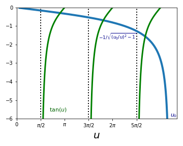
In terms of these variables, Eq. [14] reads

which can be solved numerically. One possibility is to represent graphically the tangent function together with . As indicated in the graphic below (where a value of is used), the points where these two curves cross correspond to the values of the energy that lead to solutions of Eq. [14]. In the graphic below, we indicate with vertical dashed lines the asymtotae of the tangent function.

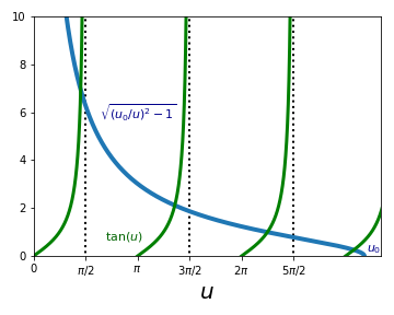
By using some numerical software, one can determine the values of and hence of for which the two functions cross and thus solve Eqns. [14] and [15]. The specific numerical values of these solutions are not particularly instructive, but it is instead useful to consider the limiting cases where the potential well is very deep, since it allows us to reproduce known results.

Note

There is a very interesting limit of the previous result. In the limit of either a very deep () or very wide potential well, we have that and you can verify that the intersections occur at values of just below the asymptotae of the tangent, that is You can convince yourselves that this result is identical to that of the infinite square well of width , which is not surprising since we are taking the limit. In this limit we have an infinite number of bound states, though for finite the number of bound states will be finite. The missing solutions of the infinite square well () will come from the odd solutions that are discussed below.

Another interesting limit is that of a narrow () or shallow () well for which . From the schematic above, we see that as decreases we will have less and less crossings (implying a reduction in the number of bound states), down to the limit where there is a single bound state (for ).

In the figure below we show schematically the wavefunction for the bound state of the potential well with the lowest energy. Note how it is indeed even under the transformation and how it falls off exponentially for large in the classically forbidden region.

Bound states with higher energy will display oscillations with higher frequencies in the well region, .

Finally, we can extend the previous derivation to the case of the odd solutions of the Schroedinger equation in the region , for which and the wave function in the region inside the potential well is given by

Imposing now the continuity of the wave function and of its first derivative at we end up with the following four equations:

Comparing the first two equations we get that , which makes the third and fourth equation identical. So, as in the case of the odd solutions, we end up with two independent equations, which can be conbined to yield

and using the same change of variables as for the even solutions we end up with the following equation:

which again can be solved numerically (and reproduces the missing solutions of the infinite potential well in the limit ). You can see below a graphical representation of this equation, with the crossings indicating the allowed values of the energy for the odd solutions of this system.

You can verify how after each even solution comes an odd solutions and viceversa. In the limit the even (odd) solutions appear at ()

Scattering states in the finite square well¶

Following this discussion of the bound states of the square potential well, we move to describe the the corresponding scattering states, defined as those states for which as indicated in the schematic below:

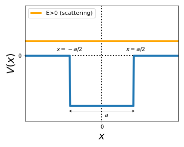
Clearly for such states we have everywhere and thus we expect to find oscillatory solutions for the wave function.

As we did in the case of the bound states, the first step is divide the problem into different regions, with each region representing a different potential. These three regions will be the same as in the previous case. Subsequently, we need to solve the Schroedinger equation separately in each of the three regions:

In this region the potential vanishes, , and making explicit that the energy is positive we end up with the following equation

which is of course nothing but the free particle Schroedinger equation that we know how to solve:

Also here the Schroedinger equation can be expressed in a way that resembles the free-particle case:

and now recalling that is symmetric and thus the wave functions in this region will be either even or odd under a transformation of the form we can express its solution as

where for even solutions and for odd solutions, in exactly the same manner as in the case of the bound states.

Now again we end up with the free particle equation

In a similar way as in the case of the scattering states for the delta potential, the interpretation of this solution is the following (see also the schematic below):

• The component represents a particle propagating from the left towards the potential well, and the component represents a particle moving towards the right way from the potential well.

• The component represents a particle propagating from the right away from the potential well, and the component represents a particle moving from the left towards the potential well.

• In the well region we have either even oscillatory functions () or odd oscillatory functions ()

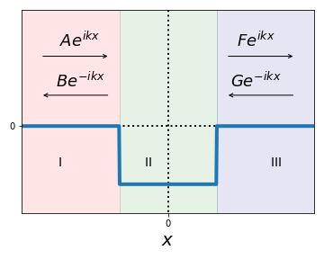
Now, as in the case of the delta function, the physically interesting case is that of a particle approaching the potential well from the left. In this configuration, , , and can be understood as the incident, transmitted, and reflected waves, and we can then set .

We can now write down the complete expression for the wave function of the finite square well for scattering states ( assuming an incident particle approaching the barrier from the left:

As we have done in the previous cases, we can try to determine the integration constants , and by means of the boundary conditions that must be satisfied by the wave function and its derivative.

• Continuity of the wavefunction:

From Eq. [16] we have

From Eq. [17] we have

• Continuity of the first derivative of the wavefunction:

From Eq. [18] we have

From Eq. [19] we have

By doing some algrebra we can rearrange these equations to obtain the following result:

In analogy with the case of the scattering states in the delta function potential, we can define a transmission and a reflection coefficients by dividing the square of the coefficients of the transmitted and reflected waves respectively by that of the incident wave.

The transmission coefficient will then be given by

As expected, ranges between 0 and 1 and its value will depend on the interplay between the particle energy and the depth and width and of the potential well.

Info

From the previous result, you can verify that for certain values of the values of the energy the probability of transmission when crossing the potential well will be unity, , which corresponds to a perfect transmission without any reflection. For these values of the energy, the potential well becomes effectively transparent. The condition for is satisfied when with an integer number, which correspond to values of the energy which is the same result as the energies of an infinite square well with width .

Finite square barrier¶

We now move to discuss the case of the finite square barrier potential. Recall that this system is defined by a potential of the from

where is a positive real number representing the height of the potential barrier and indicates its width. This potential is represented graphically in the figure below:

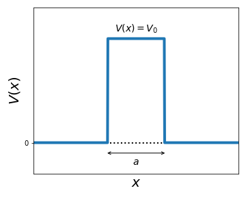
Inspection of this potential indicates that one important difference as compared to the case of the finite well is that here we cannot have bound states, and hence all allowed states will be scattering states. The reason is that we cannot have states with negative energy, and hence all states will have implying that for we have that with the oscillatory-like wave function characteristic of the scattering states.

This strategy to solve the Schroedinger equation for the finite barrier follows closely that of the finite well. Here we only sketch the main ingredients of the derivation and discuss the qualitative results expected, and leave the complete derivation as an exercise for the student.

Even if only scattering states are allowed, we need to consider two different situations:

• First, when the energy is smaller than the height of the barrier, . At the classical level, a particle with energy below the height of a potential barrier would never the able to cross it.

  However, as we will show, this is not the case in quantum theory, and an incident particle will have a finite probability to cross the barrier. This phenomenon is known as quantum tunneling.

• Second, when the energy of the particle is larger than the height of the barrier, . In this situation, classically we expect the particle to be able to cross the barrier, and in quantum theory we will see that there is indeed some probability for transmission across the barrier but also there is a finite probability for reflection.

Let us now discuss these two situations in turn.

The finite barrier for E<V0¶

Let us consider first the case for which the particle energy satisfies , which corresponds to the configuration depicted below. In this figure we also represent a characteristic wave function associated to this configuration, we will now motivate the behaviour that it exhibits.

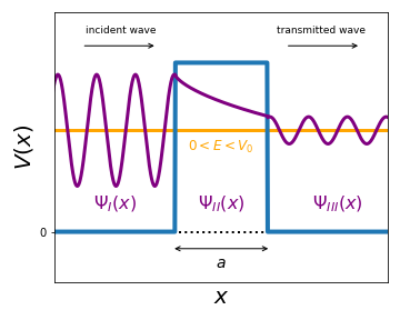
Assuming that we have an incident wave approaching the barrier from the left, you can verify that the solution of the Schroedinger equation in the three usual regions is given by (recall that in this system all energies will be positive):

The integration constants , and are related by the boundary conditions stemming from the continuity of the wave function and its derivative at . We see how in Region III the wave function oscillates with the same frequency as in Region I but with a smaller amplitude due to the fact that the barrier will reflect part of the incident wave function. In Region III, the classically forbidden region, the probability of finding the particle is non-zero but exponentially suppressed.

By analogy with the case of the scattering states in the potential well, we can compute the transmission coefficient finding that

By recalling the properties of the hyperbolic sinus , we note that in the limit (where the potential barrier becomes infinitely steep) then , implying that there is no transmitted wave and that all the incident well is reflected by the potential barrier.

Conversely, if either or , a limit in which the barrier vanishes, we obtain perfect transmission as expected.

Note

The fact that for we get a non-zero transmission coefficient, , is a most remarkable phenomenon of quantum theory known as tunneling. This means that in quantum mechanics, a particle can cross barriers in a way that is not possible in classical physics. However, we note that the probability for tunneling is exponentially suppressed and becomes negligible unless the barrier is very narrow or the energy close to .

The finite barrier for E>V0¶

Finally, we consider schematically the case for which the particle energy satisfies , which corresponds to the configuration depicted below. In this figure we also represent a characteristic wave function associated to this configuration.

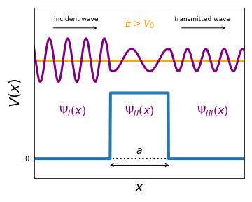
By proceeding in the usual way (solving the Schroedinger equation in each region and implementing the boundary conditions) you can convince yourselves that the qualitative behaviour of the wave function is what it should be because of the following reasons:

• In Regions I and III, the oscillation frequency of the wave is the same (same argument of ).

• In Region II, the oscillation frequency decreases since in the argument of the exponentials.

• In Region III, the amplitude of the oscillation is suppressed as compared to that of the incident wave since only part of the latter is transmitted and the rest is reflected.

Questions¶

1. A beam of electrons with total energy is incident on the potential steps from the left.

   (a) Will the beam be reflected in case A and case B? Justify your answer.

   (b) Let and denote the reflection coefficients in A and B. Is greater, smaller, or equal to ? What about compared to ? Justify your answer.

2. Two beams of electrons, A and B, with total energy of E and 2E respectively, are incident on the potential barrier from the left.

   (a) Sketch to show qualitatively the waveefunction of the two beams in all three regions. How is the wave function of the incident beam A similar to the wave function of beam B? How is it different?

   (b) Suppose the length of the barrier is increased to 2L. How will you answers be changed? How is the wave function. of beam. A in region III similar to the. wave function of beam A in region III when the length of the barrier is still L? How is it different? And how about beam B? Justify your answer.

3. Consider an electron in the potential well shown below. is the first excited state energy.

   (a) Sketch the first excited state wave function. Justify your answer.

   (b) Sketch the wave function corresponding . Justify your answer.

   (c) In both cases, where will the electron be most likely found? In each case, are there any regions that the electron will never be found? Justify your answer.

stipebestudy.blogspot.com

Source: https://qm1.quantumtinkerer.tudelft.nl/8_finite-barrier/

Share this post